Device calibrations and connectivity

Requires the latest qbraid pre-release: pip install --upgrade --pre qbraid. Calibration data is refreshed from each hardware provider roughly hourly.

Superconducting QPUs are not uniform: qubits differ in readout fidelity, and two-qubit gates only exist between physically coupled pairs, each with its own error rate. The QbraidProvider exposes both facts programmatically, so you can inspect a device before you submit to it, and place your circuit on the qubits where it will perform best.

Fetching calibration data

Every QbraidDevice has two entry points:

from qbraid.runtime import QbraidProvider

provider = QbraidProvider()
device = provider.get_device("rigetti:rigetti:qpu:cepheus-1-108q")

device.coupling_map
# ((0, 1), (0, 9), (1, 2), (1, 10), (2, 3), ...)  193 physical qubit pairs

calibration = device.get_calibrations()
calibration.last_calibrated
# '2026-07-21T20:05:45+00:00'

coupling_map is the device’s physical connectivity: sorted, deduplicated (source, target) qubit pairs, derived from the calibrated two-qubit gate edges. It is cached on the device instance, since hardware topology does not change between calibrations. get_calibrations() returns the full live snapshot and always fetches fresh data. The two most useful fields:

# Per-edge two-qubit gate error, keyed by gate name
calibration.edges["gateError"]["cz"][0]
# EdgeEntry(source=0, target=1, value=0.0246)

# Per-qubit metrics
calibration.qubits["0"]
# QubitCalibration(readout_error=0.04, gate_error={'rb': 0.0019}, ...)

Both return None for devices without published calibration data, such as simulators.

Devices with calibration data

Physical device	Qubits	Edges	Example device IDs
Rigetti Cepheus-1-108Q	107	193	`rigetti:rigetti:qpu:cepheus-1-108q`, `aws:rigetti:qpu:cepheus-1-108q`
IQM Garnet	20	30	`aws:iqm:qpu:garnet`
IQM Emerald	54	85	`aws:iqm:qpu:emerald`
AQT Ibex-Q1	12	0	`aws:aqt:qpu:ibex-q1`

All device IDs that map to the same physical hardware share one calibration snapshot, so rigetti:rigetti:qpu:cepheus-1-108q and aws:rigetti:qpu:cepheus-1-108q return identical data.

A device can have calibration data with an empty edge list. AQT’s Ibex-Q1 is a trapped-ion system with all-to-all connectivity, so there are no discrete coupling edges to report: coupling_map returns an empty tuple, not None. For IonQ trapped-ion devices, see device.profile.characterization instead.

You can also query the underlying REST endpoint directly, which works for any device ID including those not available for direct submission:

curl -H "X-API-Key: $QBRAID_API_KEY" \
  https://api.qbraid.com/api/v1/devices/rigetti:rigetti:qpu:cepheus-1-108q/calibrations

Plotting the connectivity graph

The qbraid.visualization module renders the graph in one call, colored by live calibration data. Edges are colored by two-qubit gate error and nodes by readout error, on a single-hue scale where darker is better, matching the topology view in qBraid Lab:

from qbraid.visualization import plot_connectivity_graph

plot_connectivity_graph(device)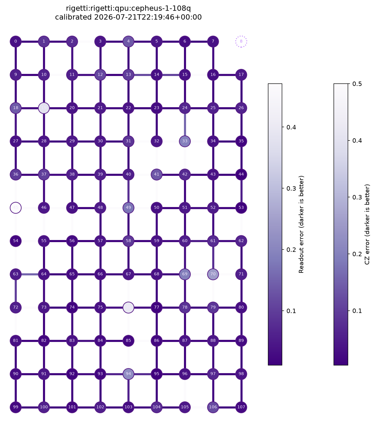

The dotted outline is a qubit in the lattice footprint with no working couplings. Light qubits and edges are the ones to avoid. The layout comes from the device document’s topology config, so square lattices (Rigetti) and clipped lattices (IQM) both render their true physical geometry; devices without a lattice config fall back to a force-directed layout. To build a custom plot, the lattice_positions helper maps qubit ids to grid coordinates from the same config:

from qbraid.visualization import lattice_positions

topology = device.client.get_device(device.id).topology
# {'type': 'square-lattice', 'rows': 12, 'cols': 9}

positions = lattice_positions(topology, range(108))
# {0: (0, 0), 1: (1, 0), ..., 107: (8, -11)}

The same call works unchanged on any device with calibration data. IQM’s Garnet renders its clipped diamond lattice:

garnet = provider.get_device("aws:iqm:qpu:garnet")
plot_connectivity_graph(garnet)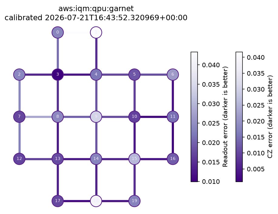

Choosing the best qubits

With the calibration data in hand, qubit selection becomes a graph problem. Build a weighted graph from the coupling map, then the single best-calibrated pair is one line:

import networkx as nx

calibration = device.get_calibrations()
edge_error = {
    (e.source, e.target): e.value
    for e in calibration.edges["gateError"]["cz"]
}

graph = nx.Graph()
for q0, q1 in device.coupling_map:
    graph.add_edge(q0, q1, error=edge_error.get((q0, q1), edge_error.get((q1, q0))))

best_edge = min(edge_error, key=edge_error.get)
# (88, 89), CZ error 0.0037 -- 2.3x better than the device median

For a linear circuit on n qubits, search for the connected chain that minimizes the summed two-qubit error:

def best_chain(graph, length):
    """Find the simple path of `length` qubits minimizing summed edge error."""
    best = (float("inf"), None)

    def extend(path, total):
        nonlocal best
        if total >= best[0]:
            return
        if len(path) == length:
            best = (total, list(path))
            return
        for nbr in graph.neighbors(path[-1]):
            if nbr not in path:
                path.append(nbr)
                extend(path, total + graph.edges[path[-2], nbr]["error"])
                path.pop()

    for start in graph.nodes:
        extend([start], 0.0)
    return best


total, chain = best_chain(graph, 5)
# chain = [88, 89, 98, 97, 96], summed CZ error 0.0214

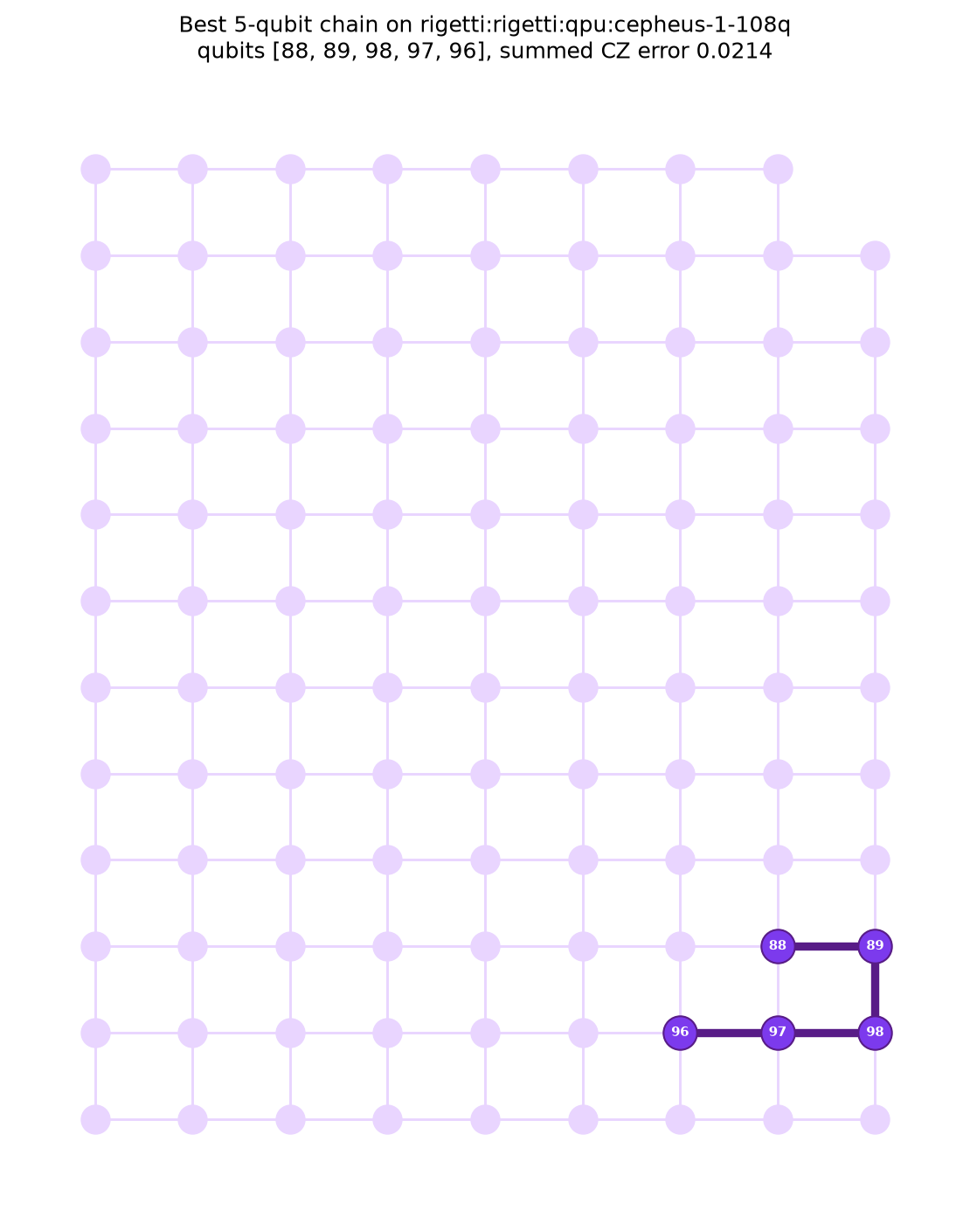
Calibrations shift with every refresh, so re-run the selection shortly before you submit. The best chain this hour is not always the best chain tonight.

Running on the qubits you chose

Rigetti direct: hand-placed native gates

On the Rigetti direct path, programs that bypass quilc must already use native gates on physical qubits, which is exactly what the coupling map enables. A Bell pair on the best-calibrated edge:

import pyquil

q0, q1 = best_edge  # (88, 89)

program = pyquil.Program(f"""
DECLARE ro BIT[2]
RX(pi/2) {q0}
RX(pi/2) {q1}
CZ {q0} {q1}
RX(-pi/2) {q1}
MEASURE {q0} ro[0]
MEASURE {q1} ro[1]
""")

job = device.run(program, shots=100)
job.wait_for_final_state()
job.result().data.get_counts()
# {'00': 44, '11': 44, '01': 7, '10': 5}  -- run on Cepheus-1-108Q, 2026-07-21

The correlated outcomes (00 and 11) came back at 88 percent on hardware, consistent with the roughly 0.4 percent CZ error and few-percent readout error of the chosen pair.

Qiskit: constrain transpilation to the real topology

If you would rather let a transpiler do the routing, feed the coupling map to Qiskit and pin your circuit to the chain you selected. This works for any gate-model device on qBraid:

from qiskit import QuantumCircuit, transpile
from qiskit.transpiler import CouplingMap

ghz = QuantumCircuit(5, 5)
ghz.h(0)
for i in range(4):
    ghz.cx(i, i + 1)
ghz.measure(range(5), range(5))

coupling = CouplingMap(
    [list(edge) for edge in garnet.coupling_map]
    + [[b, a] for a, b in garnet.coupling_map]
)
total, chain = best_chain(garnet_graph, 5)  # [6, 11, 16, 15, 10] on Garnet

transpiled = transpile(
    ghz,
    coupling_map=coupling,
    initial_layout=chain,
    basis_gates=["r", "cz"],
    optimization_level=3,
)

job = garnet.run(transpiled, shots=1000)

Every two-qubit gate in the transpiled circuit now acts on a physically coupled, well-calibrated pair, and no SWAP overhead is silently inserted for qubits you did not choose.

Transpile against the coupling map of the exact device ID you will submit to. Vendor-routed and direct device IDs share hardware and calibrations, but a circuit laid out for one device will not fit another.

QbraidProvider: setup and credentials
Rigetti Cepheus-1-108Q: native gates, Quil-T timing, and the two compilation paths
Job execution: single, batch, and group submission
Visualization: histograms and other built-in plotting utilities

User Guide

API Reference

Device calibrations and connectivity

Fetching calibration data

Devices with calibration data

Plotting the connectivity graph

Choosing the best qubits

Running on the qubits you chose

Rigetti direct: hand-placed native gates

Qiskit: constrain transpilation to the real topology

​Fetching calibration data

​Devices with calibration data

​Plotting the connectivity graph

​Choosing the best qubits

​Running on the qubits you chose

​Rigetti direct: hand-placed native gates

​Qiskit: constrain transpilation to the real topology

​Related links

Fetching calibration data

Devices with calibration data

Plotting the connectivity graph

Choosing the best qubits

Running on the qubits you chose

Rigetti direct: hand-placed native gates

Qiskit: constrain transpilation to the real topology

Related links