> ## Documentation Index
> Fetch the complete documentation index at: https://docs.qbraid.com/llms.txt
> Use this file to discover all available pages before exploring further.
# Visualization
> Draw circuit diagrams and plot experimental results, conversion graphs, and more.
API Reference:
[qbraid.visualization](https://qbraid.github.io/qBraid/api/qbraid.visualization.html)
## Draw Circuit Diagrams
qBraid's `circuit_drawer` function takes in any type of supported quantum circuit and draws the corresponding visualization.
Here's an example using `braket` and `cirq`:
```python theme={null}
from qbraid import random_circuit
from qbraid.visualization import circuit_drawer
circuit = random_circuit("braket")
circuit_drawer(circuit)
# T : |0| 1 |2|
#
# q0 : -C-C---S-
# | |
# q1 : -Z-|-Z---
# |
# q2 : -Z-X-----
#
# T : |0| 1 |2|
circuit = random_circuit("cirq")
circuit_drawer(circuit)
# 0: ───────────×───Z───
# │
# 1: ───iSwap───×───────
# │
# 2: ───iSwap───Y───H───
```
### Draw OpenQASM 3 circuits
The `circuit_drawer` function accepts a string of OpenQASM 3 code and returns a matplotlib figure of the circuit:
```python theme={null}
from qbraid.visualization import circuit_drawer
program = """
OPENQASM 3;
include "stdgates.inc";
qubit[2] q;
h q[0];
cx q[0], q[1];
"""
circuit_drawer(program)
```
**Note**: The above is the equivalent to calling `pyqasm.draw(..., output="mpl")`
## Plot Experimental Results
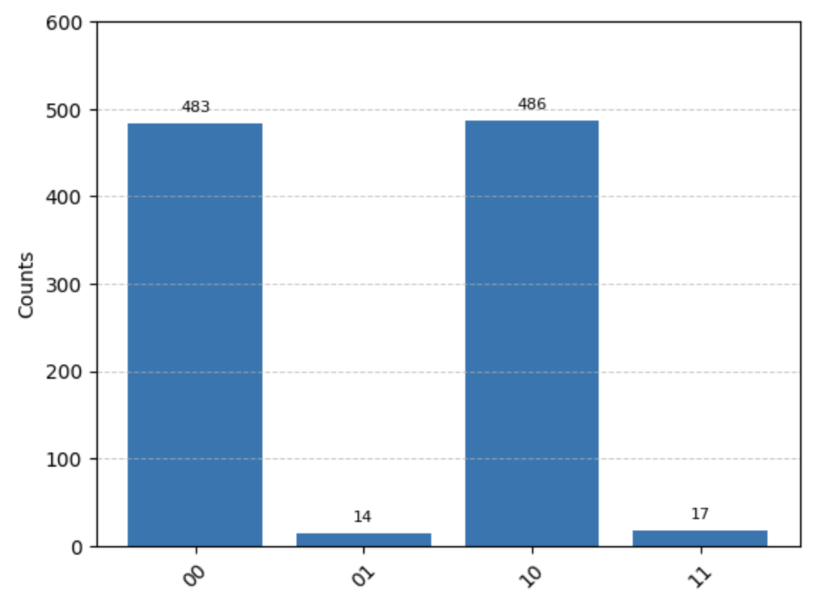
Gather the measurement counts and plot the histogram data for any `Result` constructed from `ResultData` of type `qbraid.runtime.GateModelResultData`:
```python theme={null}
from qbraid.visualization import plot_histogram
counts = result.data.get_counts()
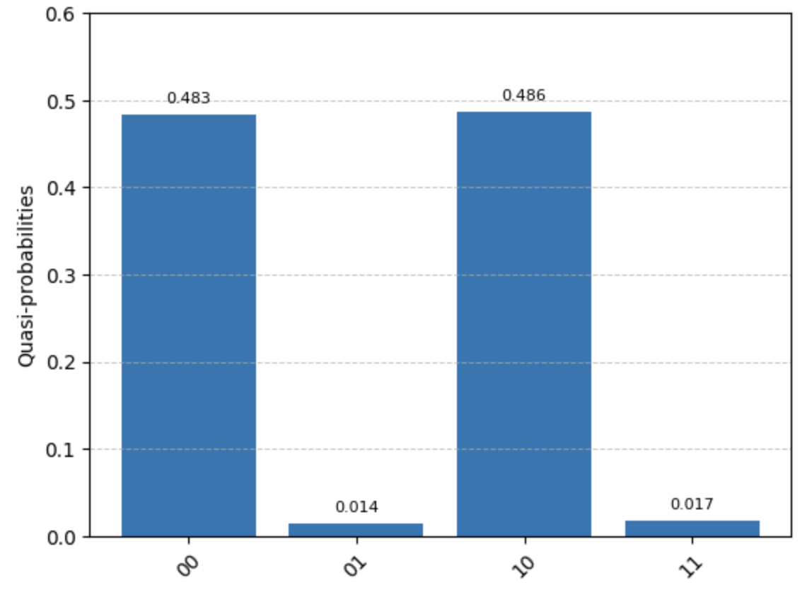
# {'00': 483, '01': 14, '10': 486, '11': 17}
plot_histogram(counts)
```
Or, using the same measurement counts data, plot the probability distribution:
```python theme={null}
from qbraid.visualization plot_distribution
plot_distribution(counts)
```
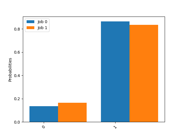
Or, plot a batch of measurement counts for any `list[qbraid.runtime.GateModeResultData]`:
```python theme={null}
batch_jobs = device.run_batch([circuit0, circuit1], shots=1000)
batch_results = [job.result() for job in batch_jobs]
batch_counts = [result.data.get_counts() for result in batch_results]
# e.g. [{'0': 136, '1': 864}, {'0': 166, '1': 834}]
plot_histogram(batch_counts)
```
Using the qBraid runtime job and results primitives, experimental data is returned in a standardized format,
facilitating straightforward comparisons and benchmarking of results across different providers and backends.
## Plot Transpiler Conversions
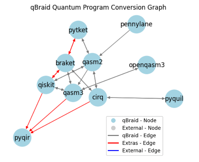
Plot all supported conversions between registered program types available through the `qbraid.transpiler`:
```python theme={null}
from qbraid import ConversionGraph
from qbraid.visualization import plot_conversion_graph
graph = ConversionGraph()
plot_conversion_graph(graph, legend=True)
```
## Plot Runtime Conversion Scheme
Plot the runtime conversion scheme for any `qbraid.runtime.QuantumDevice`.
The `QuantumDevice.scheme` defines the `qbraid.transpiler.ConversionScheme` that will be used to carry out the "transpile" step of the [Quantum Job Submission Process](/v2/sdk/user-guide/runtime/components#quantum-job-submission-process).
```python theme={null}
from qbraid import QbraidProvider
from qbraid.visualization import plot_runtime_conversion_scheme
provider = QbraidProvider()
device = provider.get_device("qbraid:qbraid:sim:qir-sv")
print(device.scheme)
```
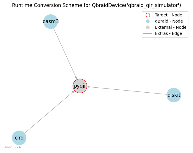
By setting the maximum path depth to 1, we ensure the `ConversionGraph` includes only program types (nodes) that are directly connected to the target program type by a single conversion step (edge).
```python theme={null}
device.update_scheme(max_path_depth=1)
plot_runtime_conversion_scheme(device)
```
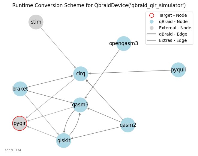
By setting the maximum path depth to 2, we can see how the `ConversionGraph` is expanded to include program types (nodes) that are at most two conversion steps (edges) away from the target program type.
```python theme={null}
device.update_scheme(max_path_depth=2)
plot_runtime_conversion_scheme(device)
```