> ## Documentation Index
> Fetch the complete documentation index at: https://docs.qbraid.com/llms.txt
> Use this file to discover all available pages before exploring further.
# Fire Opal
> Environment for developing with Fire Opal, a Python package containing a large suite of error suppression techniques intended to improve the quality of quantum algorithm results.
# Overview
[Fire Opal](https://q-ctrl.com/fire-opal) is a software package that makes it simple for anyone to achieve meaningful results from quantum computers. Using AI-driven error suppression, Fire Opal improves the success of algorithms by thousands of times and enables you to successfully scale to large problem sizes, without even having to worry about the details of quantum circuits. At the same time, reaching the correct answer takes fewer shots and requires no overhead, meaning that you save on compute cost. For an in-depth explanation of Fire Opal's benefits and capabilities, check out the Fire Opal overview.
This tutorial will run through the steps to set up Fire Opal on the qBraid Lab platform and use it to run a Bernstein-Vazirani circuit. After completion, you will have demonstrated Fire Opal's benefits by comparing the success probabilities of executing the circuit with both Fire Opal and Qiskit.
Click below to clone the [qbraid-lab-demo](https://github.com/qBraid/qbraid-lab-demo) repository into your qBraid Lab, and then open `qbraid_lab` > `fire_opal` > `get-started.ipynb` to follow along with the code examples in this tutorial.
 # Setup
## 1. Sign up for Q-CTRL account
You will need to [sign up for a Q-CTRL account](https://q-ctrl.com/fire-opal) to run the Fire Opal package.
## 2. Install the Fire Opal Environment in qBraid Lab
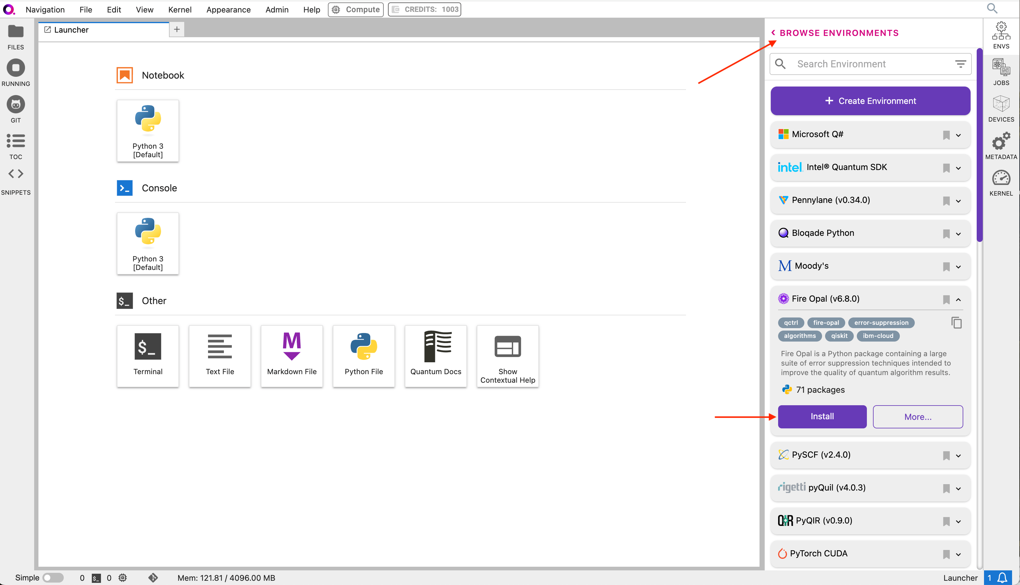
2a. In the Environment Manager sidebar, click **Add** to view the environments available to install.
2b. Choose the Fire Opal environment, expand its panel, and click **Install**.
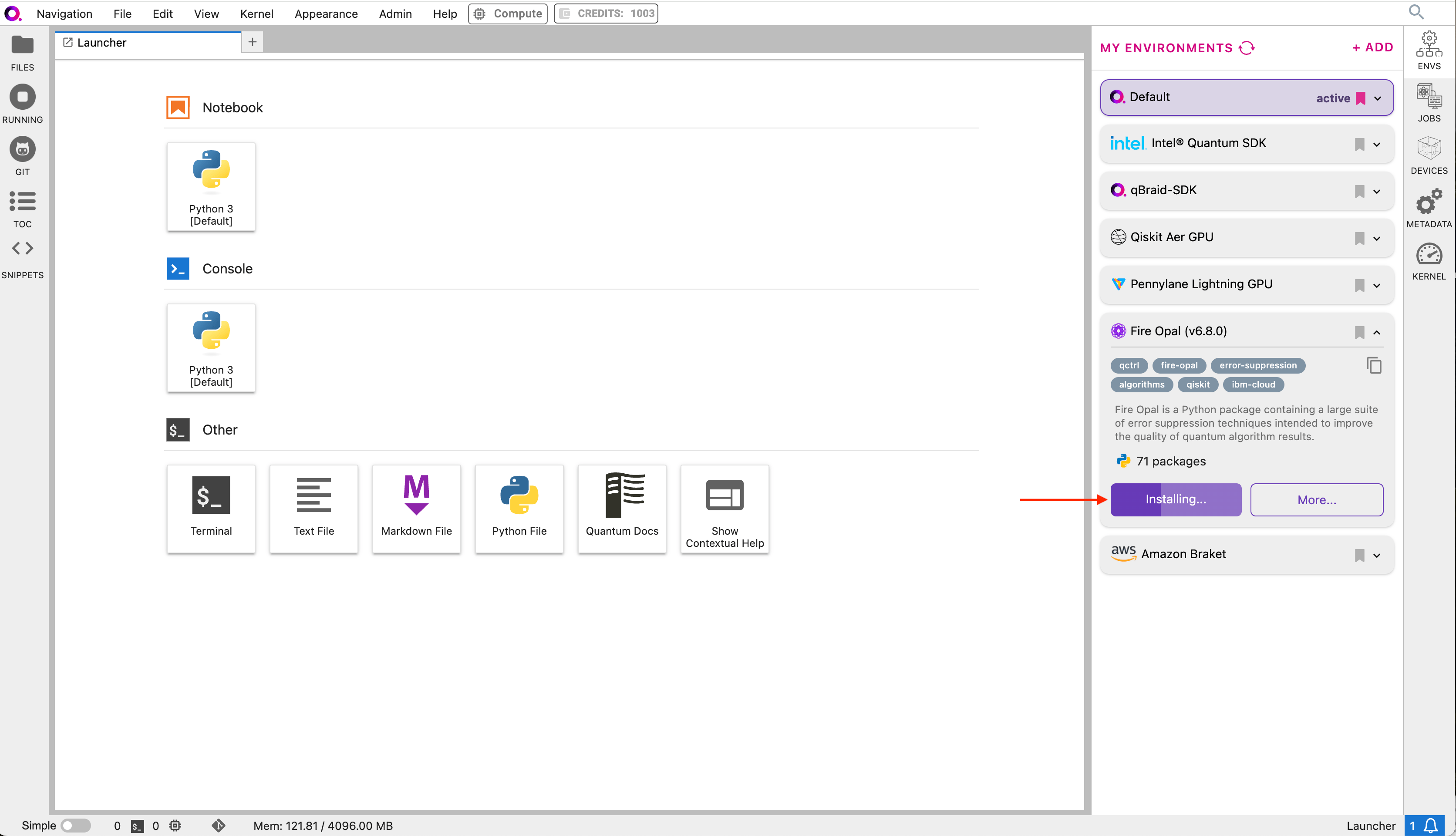
2c. Once the installation has started, the panel is moved to the **My Environments** tab. Click **Browse Environments** to return to the **My Environments** tab and view its progress.
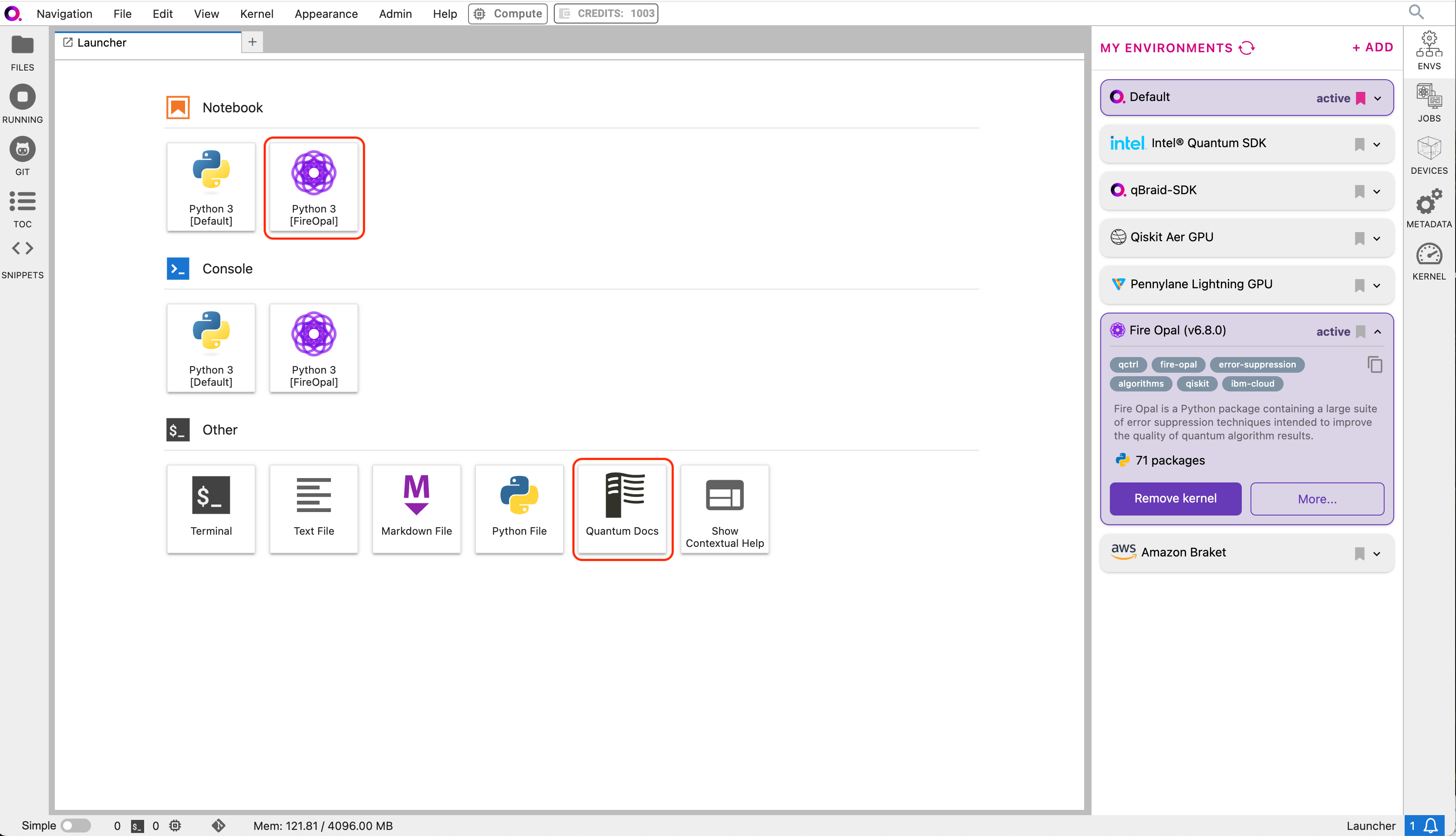
2d. When the installation is complete, the environment panel's action button will switch from **Installing…** to **Add Kernel**.
Click **Add Kernel** and open a new notebook to beginning coding with the Fire Opal environment. You can also click the **Quantum Docs**
icon to browse the integrated Fire Opal documentation.
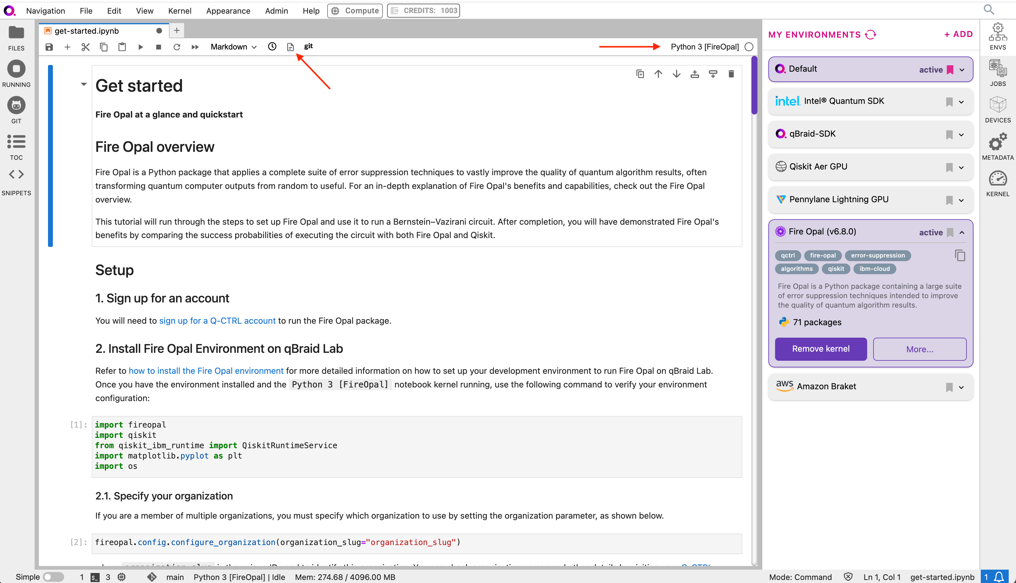
2e. In the new notebook, make sure that your ipykernel (top-right) is set to `Python 3 [FireOpal]`
(see [switch notebook kernel](/v2/lab/user-guide/notebooks/#switch-notebook-kernel)). Then, verify that the Fire Opal environment
is configured correctly by running the following code in the first cell:
```python theme={null}
import fireopal
import qiskit
from qiskit_ibm_runtime import QiskitRuntimeService
import matplotlib.pyplot as plt
import os
```
When you have the Fire Opal kernel selected, clicking the docs link in the notebook top-bar will take you directly to the Fire Opal
documentation page in a new tab.
2f. You are now ready to use Fire Opal in the qBraid Lab environment! Finish setup by configuring your Q-CTRL organization and
IBM Cloud credentials, and then follow the tutorial below to run a Bernstein-Vazirani circuit.
## 3. Specify your Q-CTRL organization
If you are a member of multiple organizations, you must specify which organization to use by setting the organization parameter,
as shown below.
```python theme={null}
fireopal.config.configure_organization(organization_slug="organization_slug")
```
where `organization_slug` is the unique ID used to identify this organization. You can check organization names and other
details by visiting your [Q-CTRL account](https://accounts.q-ctrl.com/).
## 4. Sign up for an IBM Cloud account
While Fire Opal's technology is inherently backend agnostic, in this tutorial we will run the circuit on an IBM Quantum backend device.
You will need to sign up for an [IBM Quantum account](https://quantum.cloud.ibm.com/signin?redirectTo=%2F), which you can
use to access devices on the Open or Premium IBM Quantum plans. Simply input your hub, group, project, and access token to the
[make\_credentials\_for\_ibm\_cloud](https://docs.q-ctrl.com/references/fire-opal/fireopal/fireopal.credentials.make_credentials_for_ibm_cloud#fireopal.credentials.make_credentials_for_ibm_cloud)
function.
IBM Quantum offers public access to some of their quantum computers. However,
queue times for public systems can be long, which will cause delays in the
execution steps of this guide (demo steps 5 and 7). These delays are
extraneous to Fire Opal.
# Demo: Running the Bernstein-Vazirani algorithm with Fire Opal
We’ll use Fire Opal to run a Bernstein-Vazirani circuit. This algorithm is broadly used to find a string from the outputs of a
black box function, though this information is not necessary for the sake of running this example.
## 1. Define helper functions
* `draw_circuit`: draws our QASM circuit
* `plot_bv_results`: plots the results of our experiments
```python theme={null}
shot_count = 2048
def draw_circuit(qasm_str: str):
"""Draws a QASM circuit."""
circuit = qiskit.QuantumCircuit.from_qasm_str(qasm_str)
display(circuit.draw(fold=-1))
def plot_bv_results(results, hidden_string, title=""):
"""Plot a probability histogram and highlight the hidden string."""
bitstrings = sorted(results.keys())
def to_probability(value, total):
if isinstance(value, float):
return value
return value / total
probabilities = [to_probability(results[b], shot_count) for b in bitstrings]
plt.figure(figsize=(50, 5))
bars = plt.bar(bitstrings, probabilities)
plt.xticks(rotation=90)
for index, bitstring in enumerate(bitstrings):
if bitstring != hidden_string:
bars[index].set_color("grey")
plt.ylabel("Probability")
plt.ylim([0, 1])
plt.title(title)
plt.show()
```
## 2. Provider the quantum circuit
Here, we will define the Bernstein-Vazirani circuit as an [OpenQASM](https://openqasm.com/) string and visualize it using our
previously defined helper function `draw_circuit`. Such a string can also be generated by exporting a quantum circuit written
with any quantum-specific Python library.
```python theme={null}
circuit_qasm = """OPENQASM 2.0;
include "qelib1.inc";
qreg q[12];
creg c[11];
x q[11];
h q[0];
h q[1];
h q[2];
h q[3];
h q[4];
h q[5];
h q[6];
h q[7];
h q[8];
h q[9];
h q[10];
h q[11];
barrier q[0],q[1],q[2],q[3],q[4],q[5],q[6],q[7],q[8],q[9],q[10],q[11];
cx q[0],q[11];
cx q[1],q[11];
cx q[2],q[11];
cx q[3],q[11];
cx q[4],q[11];
cx q[5],q[11];
cx q[6],q[11];
cx q[7],q[11];
cx q[8],q[11];
cx q[9],q[11];
cx q[10],q[11];
barrier q[0],q[1],q[2],q[3],q[4],q[5],q[6],q[7],q[8],q[9],q[10],q[11];
h q[0];
h q[1];
h q[2];
h q[3];
h q[4];
h q[5];
h q[6];
h q[7];
h q[8];
h q[9];
h q[10];
h q[11];
barrier q[0],q[1],q[2],q[3],q[4],q[5],q[6],q[7],q[8],q[9],q[10],q[11];
measure q[0] -> c[0];
measure q[1] -> c[1];
measure q[2] -> c[2];
measure q[3] -> c[3];
measure q[4] -> c[4];
measure q[5] -> c[5];
measure q[6] -> c[6];
measure q[7] -> c[7];
measure q[8] -> c[8];
measure q[9] -> c[9];
measure q[10] -> c[10];
"""
draw_circuit(circuit_qasm)
```
```
┌───┐ ░ ░ ┌───┐ ░ ┌─┐
q_0: ┤ H ├──────░───■─────────────────────────────────────────────────────░─┤ H ├─░─┤M├──────────────────────────────
├───┤ ░ │ ░ ├───┤ ░ └╥┘┌─┐
q_1: ┤ H ├──────░───┼────■────────────────────────────────────────────────░─┤ H ├─░──╫─┤M├───────────────────────────
├───┤ ░ │ │ ░ ├───┤ ░ ║ └╥┘┌─┐
q_2: ┤ H ├──────░───┼────┼────■───────────────────────────────────────────░─┤ H ├─░──╫──╫─┤M├────────────────────────
├───┤ ░ │ │ │ ░ ├───┤ ░ ║ ║ └╥┘┌─┐
q_3: ┤ H ├──────░───┼────┼────┼────■──────────────────────────────────────░─┤ H ├─░──╫──╫──╫─┤M├─────────────────────
├───┤ ░ │ │ │ │ ░ ├───┤ ░ ║ ║ ║ └╥┘┌─┐
q_4: ┤ H ├──────░───┼────┼────┼────┼────■─────────────────────────────────░─┤ H ├─░──╫──╫──╫──╫─┤M├──────────────────
├───┤ ░ │ │ │ │ │ ░ ├───┤ ░ ║ ║ ║ ║ └╥┘┌─┐
q_5: ┤ H ├──────░───┼────┼────┼────┼────┼────■────────────────────────────░─┤ H ├─░──╫──╫──╫──╫──╫─┤M├───────────────
├───┤ ░ │ │ │ │ │ │ ░ ├───┤ ░ ║ ║ ║ ║ ║ └╥┘┌─┐
q_6: ┤ H ├──────░───┼────┼────┼────┼────┼────┼────■───────────────────────░─┤ H ├─░──╫──╫──╫──╫──╫──╫─┤M├────────────
├───┤ ░ │ │ │ │ │ │ │ ░ ├───┤ ░ ║ ║ ║ ║ ║ ║ └╥┘┌─┐
q_7: ┤ H ├──────░───┼────┼────┼────┼────┼────┼────┼────■──────────────────░─┤ H ├─░──╫──╫──╫──╫──╫──╫──╫─┤M├─────────
├───┤ ░ │ │ │ │ │ │ │ │ ░ ├───┤ ░ ║ ║ ║ ║ ║ ║ ║ └╥┘┌─┐
q_8: ┤ H ├──────░───┼────┼────┼────┼────┼────┼────┼────┼────■─────────────░─┤ H ├─░──╫──╫──╫──╫──╫──╫──╫──╫─┤M├──────
├───┤ ░ │ │ │ │ │ │ │ │ │ ░ ├───┤ ░ ║ ║ ║ ║ ║ ║ ║ ║ └╥┘┌─┐
q_9: ┤ H ├──────░───┼────┼────┼────┼────┼────┼────┼────┼────┼────■────────░─┤ H ├─░──╫──╫──╫──╫──╫──╫──╫──╫──╫─┤M├───
├───┤ ░ │ │ │ │ │ │ │ │ │ │ ░ ├───┤ ░ ║ ║ ║ ║ ║ ║ ║ ║ ║ └╥┘┌─┐
q_10: ┤ H ├──────░───┼────┼────┼────┼────┼────┼────┼────┼────┼────┼────■───░─┤ H ├─░──╫──╫──╫──╫──╫──╫──╫──╫──╫──╫─┤M├
├───┤┌───┐ ░ ┌─┴─┐┌─┴─┐┌─┴─┐┌─┴─┐┌─┴─┐┌─┴─┐┌─┴─┐┌─┴─┐┌─┴─┐┌─┴─┐┌─┴─┐ ░ ├───┤ ░ ║ ║ ║ ║ ║ ║ ║ ║ ║ ║ └╥┘
q_11: ┤ X ├┤ H ├─░─┤ X ├┤ X ├┤ X ├┤ X ├┤ X ├┤ X ├┤ X ├┤ X ├┤ X ├┤ X ├┤ X ├─░─┤ H ├─░──╫──╫──╫──╫──╫──╫──╫──╫──╫──╫──╫─
└───┘└───┘ ░ └───┘└───┘└───┘└───┘└───┘└───┘└───┘└───┘└───┘└───┘└───┘ ░ └───┘ ░ ║ ║ ║ ║ ║ ║ ║ ║ ║ ║ ║
c: 11/════════════════════════════════════════════════════════════════════════════════╩══╩══╩══╩══╩══╩══╩══╩══╩══╩══╩═
0 1 2 3 4 5 6 7 8 9 10
```
## 3. Provide your device information and credentials
Next, we'll provide device information for the real hardware backend. Fire Opal will execute the circuit on the backend on your
behalf, and it is designed to work seamlessly across multiple backend providers. For this example, we will use an IBM Quantum
hardware device.
Note that the code below requires your IBM Quantum API token. Visit [IBM Quantum](https://quantum.ibm.com/) to sign up for an
account and [obtain your access credentials](https://docs.quantum-computing.ibm.com/run/account-management).
```python theme={null}
# These are the properties for the publicly available provider for IBM backends.
# If you have access to a private provider and wish to use it, replace these values.
hub = "ibm-q"
group = "open"
project = "main"
token = "YOUR_IBM_TOKEN"
credentials = fireopal.credentials.make_credentials_for_ibmq(
token=token, hub=hub, group=group, project=project
)
QiskitRuntimeService.save_account(
token, instance=hub + "/" + group + "/" + project, overwrite=True
)
service = QiskitRuntimeService()
```
Next we will use the function `show_supported_devices` to list the devices that are both supported by Fire Opal and accessible
to you when using the `credentials` above.
```python theme={null}
supported_devices = fireopal.show_supported_devices(credentials=credentials)[
"supported_devices"
]
for name in supported_devices:
print(name)
```
From the resulting list, you can choose a backend device and replace `"desired_backend"`. The list will only include devices
accessible to you.
```python theme={null}
# Enter your desired IBM backend here or select one with a small queue
backend_name = "desired_backend"
print(f"Will run on backend: {backend_name}")
```
## 4. Validate the circuit and backend
Now that we have defined our credentials and are able to select a device we wish to use, we can validate that Fire Opal can
compile our circuit, and that it’s compatible with the indicated backend.
```python theme={null}
validate_results = fireopal.validate(
circuits=[circuit_qasm], credentials=credentials, backend_name=backend_name
)
if validate_results["results"] == []:
print("No errors found.")
else:
print("The following errors were found:")
for error in validate_results["results"]:
print(error)
```
In this previous example, the output should be an empty list since there are no errors in the circuit, i.e.
`validate_results["results"] == []`. Note that the length of the `validate_results` list is the total number of errors present
across all circuits in a batch. Since our circuit is error free, we can execute our circuit on real hardware.
## 5. Execute the circuit using Fire Opal
In the absence of hardware noise, only a single experiment would be required to obtain the correct hidden string: `111 111 111 11`.
However in real quantum hardware, noise disturbs the state of the system and degrades performance, decreasing the probability of
obtaining the correct answer for any single experiment. Fire Opal automates the adjustments made by experts when running circuits
on a real device.
Once jobs are submitted, there may be a delay in returning results due to the
hardware provider's queue. You can [view and retrieve results
later](https://docs.q-ctrl.com/fire-opal/user-guides/how-to-view-previous-jobs-and-retrieve-results).
Be sure to let your jobs finish executing, and do not cancel the process. Even
in the case of kernel disconnection, the job will still complete, and results
can later be retrieved.
```python theme={null}
print(
"Submitted the circuit to IBM. Note: there may be a delay in getting results due to IBM "
"device queues. Check the status through instructions at "
"https://cloud.ibm.com/docs/quantum-computing?topic=quantum-computing-results."
)
real_hardware_results = fireopal.execute(
circuits=[circuit_qasm],
shot_count=shot_count,
credentials=credentials,
backend_name=backend_name,
)
bitstring_results = real_hardware_results["results"]
```
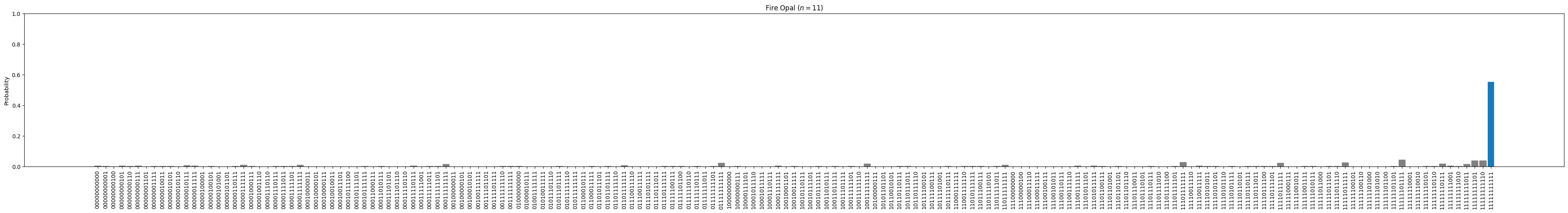
## 6. Analyze Results
Now you can look at the outputs from the quantum circuit executions. The success probability is simply the number of times the
hidden string was obtained out of the total number of circuit shots. For reference, running this circuit on a real device without
Fire Opal typically has a success probability of 2-3%. As you can see, Fire Opal greatly improved the success probability.
```python theme={null}
print(f"Success probability: {100 * bitstring_results[0]['11111111111']:.2f}%")
# Success probability: 55.19%
```
```python theme={null}
plot_bv_results(
bitstring_results[0], hidden_string="11111111111", title=f"Fire Opal ($n=11$)"
)
```
## 7. Compare Fire Opal Results with Qiskit
To get a true comparison, let's run the same circuit without Fire Opal. We'll run the circuit using Qiskit on the same IBM
backend as used previously to get a one-to-one comparison.
```python theme={null}
from qiskit_ibm_runtime import Sampler, Options
backend = service.backend(backend_name)
options = Options()
options.execution.shots = shot_count
sampler = Sampler(backend=backend, options=options)
circuit_qiskit = qiskit.QuantumCircuit.from_qasm_str(circuit_qasm)
ibm_result = sampler.run(circuit_qiskit).result()
ibm_probabilities = (
ibm_result.quasi_dists[0]
.nearest_probability_distribution()
.binary_probabilities(num_bits=11)
)
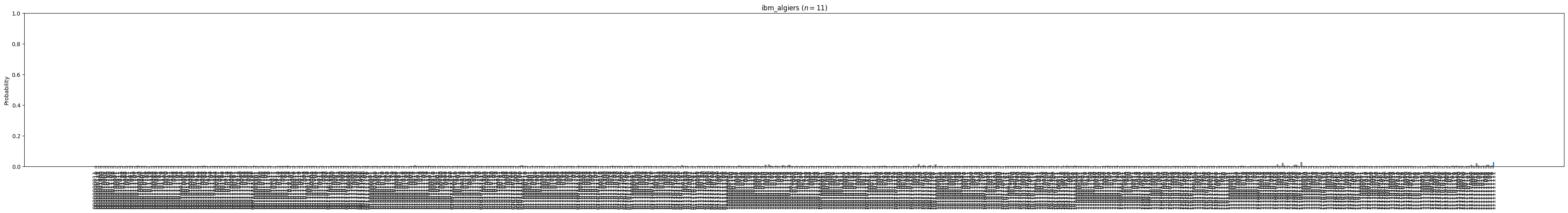
print(f"Success probability: {100 * ibm_probabilities['11111111111']:.2f}%")
# Success probability: 2.78%
```
```python theme={null}
plot_bv_results(
ibm_probabilities, hidden_string="11111111111", title=f"{backend_name} ($n=11$)"
)
```
The above results demonstrate that noise has severely impacted the probability of obtaining the correct hidden string as the output.
In this case, the string returned with the greatest frequency by the quantum computer was not the expected `111 111 111 11` state.
We should also take note of the amount of incorrect states that now contain non-zero return probabilities. Not only do default
configurations fail to find the correct answer, they also increase the probabilities of the incorrect answers.
In fact, the performance degradation is so severe that in order to be reasonably sure of the hidden string, using the original
classical algorithm would be more efficient.
You can tell that Fire Opal found the correct answer because the mode of the output distribution, or the most frequent outcome,
matches the desired output: bitstring `111 111 111 11`. Fire Opal significantly improves the probability of a successful outcome,
often by a factor of ten or more.
```python theme={null}
fire_opal_success = bitstring_results[0]["11111111111"]
ibm_success = ibm_probabilities["11111111111"]
factor = int(fire_opal_success / ibm_success)
print(f"Fire Opal improved success probability by a factor of {factor}!")
# Fire Opal improved success probability by a factor of 19!
```
Congratulations! You've run your first algorithm with Fire Opal and demonstrated its ability in transforming a device which
finds the incorrect answer by default, to a device that finds the correct answer.
Fire Opal Documentation
# Setup
## 1. Sign up for Q-CTRL account
You will need to [sign up for a Q-CTRL account](https://q-ctrl.com/fire-opal) to run the Fire Opal package.
## 2. Install the Fire Opal Environment in qBraid Lab
2a. In the Environment Manager sidebar, click **Add** to view the environments available to install.
2b. Choose the Fire Opal environment, expand its panel, and click **Install**.
2c. Once the installation has started, the panel is moved to the **My Environments** tab. Click **Browse Environments** to return to the **My Environments** tab and view its progress.
2d. When the installation is complete, the environment panel's action button will switch from **Installing…** to **Add Kernel**.
Click **Add Kernel** and open a new notebook to beginning coding with the Fire Opal environment. You can also click the **Quantum Docs**
icon to browse the integrated Fire Opal documentation.
2e. In the new notebook, make sure that your ipykernel (top-right) is set to `Python 3 [FireOpal]`
(see [switch notebook kernel](/v2/lab/user-guide/notebooks/#switch-notebook-kernel)). Then, verify that the Fire Opal environment
is configured correctly by running the following code in the first cell:
```python theme={null}
import fireopal
import qiskit
from qiskit_ibm_runtime import QiskitRuntimeService
import matplotlib.pyplot as plt
import os
```
When you have the Fire Opal kernel selected, clicking the docs link in the notebook top-bar will take you directly to the Fire Opal
documentation page in a new tab.
2f. You are now ready to use Fire Opal in the qBraid Lab environment! Finish setup by configuring your Q-CTRL organization and
IBM Cloud credentials, and then follow the tutorial below to run a Bernstein-Vazirani circuit.
## 3. Specify your Q-CTRL organization
If you are a member of multiple organizations, you must specify which organization to use by setting the organization parameter,
as shown below.
```python theme={null}
fireopal.config.configure_organization(organization_slug="organization_slug")
```
where `organization_slug` is the unique ID used to identify this organization. You can check organization names and other
details by visiting your [Q-CTRL account](https://accounts.q-ctrl.com/).
## 4. Sign up for an IBM Cloud account
While Fire Opal's technology is inherently backend agnostic, in this tutorial we will run the circuit on an IBM Quantum backend device.
You will need to sign up for an [IBM Quantum account](https://quantum.cloud.ibm.com/signin?redirectTo=%2F), which you can
use to access devices on the Open or Premium IBM Quantum plans. Simply input your hub, group, project, and access token to the
[make\_credentials\_for\_ibm\_cloud](https://docs.q-ctrl.com/references/fire-opal/fireopal/fireopal.credentials.make_credentials_for_ibm_cloud#fireopal.credentials.make_credentials_for_ibm_cloud)
function.
IBM Quantum offers public access to some of their quantum computers. However,
queue times for public systems can be long, which will cause delays in the
execution steps of this guide (demo steps 5 and 7). These delays are
extraneous to Fire Opal.
# Demo: Running the Bernstein-Vazirani algorithm with Fire Opal
We’ll use Fire Opal to run a Bernstein-Vazirani circuit. This algorithm is broadly used to find a string from the outputs of a
black box function, though this information is not necessary for the sake of running this example.
## 1. Define helper functions
* `draw_circuit`: draws our QASM circuit
* `plot_bv_results`: plots the results of our experiments
```python theme={null}
shot_count = 2048
def draw_circuit(qasm_str: str):
"""Draws a QASM circuit."""
circuit = qiskit.QuantumCircuit.from_qasm_str(qasm_str)
display(circuit.draw(fold=-1))
def plot_bv_results(results, hidden_string, title=""):
"""Plot a probability histogram and highlight the hidden string."""
bitstrings = sorted(results.keys())
def to_probability(value, total):
if isinstance(value, float):
return value
return value / total
probabilities = [to_probability(results[b], shot_count) for b in bitstrings]
plt.figure(figsize=(50, 5))
bars = plt.bar(bitstrings, probabilities)
plt.xticks(rotation=90)
for index, bitstring in enumerate(bitstrings):
if bitstring != hidden_string:
bars[index].set_color("grey")
plt.ylabel("Probability")
plt.ylim([0, 1])
plt.title(title)
plt.show()
```
## 2. Provider the quantum circuit
Here, we will define the Bernstein-Vazirani circuit as an [OpenQASM](https://openqasm.com/) string and visualize it using our
previously defined helper function `draw_circuit`. Such a string can also be generated by exporting a quantum circuit written
with any quantum-specific Python library.
```python theme={null}
circuit_qasm = """OPENQASM 2.0;
include "qelib1.inc";
qreg q[12];
creg c[11];
x q[11];
h q[0];
h q[1];
h q[2];
h q[3];
h q[4];
h q[5];
h q[6];
h q[7];
h q[8];
h q[9];
h q[10];
h q[11];
barrier q[0],q[1],q[2],q[3],q[4],q[5],q[6],q[7],q[8],q[9],q[10],q[11];
cx q[0],q[11];
cx q[1],q[11];
cx q[2],q[11];
cx q[3],q[11];
cx q[4],q[11];
cx q[5],q[11];
cx q[6],q[11];
cx q[7],q[11];
cx q[8],q[11];
cx q[9],q[11];
cx q[10],q[11];
barrier q[0],q[1],q[2],q[3],q[4],q[5],q[6],q[7],q[8],q[9],q[10],q[11];
h q[0];
h q[1];
h q[2];
h q[3];
h q[4];
h q[5];
h q[6];
h q[7];
h q[8];
h q[9];
h q[10];
h q[11];
barrier q[0],q[1],q[2],q[3],q[4],q[5],q[6],q[7],q[8],q[9],q[10],q[11];
measure q[0] -> c[0];
measure q[1] -> c[1];
measure q[2] -> c[2];
measure q[3] -> c[3];
measure q[4] -> c[4];
measure q[5] -> c[5];
measure q[6] -> c[6];
measure q[7] -> c[7];
measure q[8] -> c[8];
measure q[9] -> c[9];
measure q[10] -> c[10];
"""
draw_circuit(circuit_qasm)
```
```
┌───┐ ░ ░ ┌───┐ ░ ┌─┐
q_0: ┤ H ├──────░───■─────────────────────────────────────────────────────░─┤ H ├─░─┤M├──────────────────────────────
├───┤ ░ │ ░ ├───┤ ░ └╥┘┌─┐
q_1: ┤ H ├──────░───┼────■────────────────────────────────────────────────░─┤ H ├─░──╫─┤M├───────────────────────────
├───┤ ░ │ │ ░ ├───┤ ░ ║ └╥┘┌─┐
q_2: ┤ H ├──────░───┼────┼────■───────────────────────────────────────────░─┤ H ├─░──╫──╫─┤M├────────────────────────
├───┤ ░ │ │ │ ░ ├───┤ ░ ║ ║ └╥┘┌─┐
q_3: ┤ H ├──────░───┼────┼────┼────■──────────────────────────────────────░─┤ H ├─░──╫──╫──╫─┤M├─────────────────────
├───┤ ░ │ │ │ │ ░ ├───┤ ░ ║ ║ ║ └╥┘┌─┐
q_4: ┤ H ├──────░───┼────┼────┼────┼────■─────────────────────────────────░─┤ H ├─░──╫──╫──╫──╫─┤M├──────────────────
├───┤ ░ │ │ │ │ │ ░ ├───┤ ░ ║ ║ ║ ║ └╥┘┌─┐
q_5: ┤ H ├──────░───┼────┼────┼────┼────┼────■────────────────────────────░─┤ H ├─░──╫──╫──╫──╫──╫─┤M├───────────────
├───┤ ░ │ │ │ │ │ │ ░ ├───┤ ░ ║ ║ ║ ║ ║ └╥┘┌─┐
q_6: ┤ H ├──────░───┼────┼────┼────┼────┼────┼────■───────────────────────░─┤ H ├─░──╫──╫──╫──╫──╫──╫─┤M├────────────
├───┤ ░ │ │ │ │ │ │ │ ░ ├───┤ ░ ║ ║ ║ ║ ║ ║ └╥┘┌─┐
q_7: ┤ H ├──────░───┼────┼────┼────┼────┼────┼────┼────■──────────────────░─┤ H ├─░──╫──╫──╫──╫──╫──╫──╫─┤M├─────────
├───┤ ░ │ │ │ │ │ │ │ │ ░ ├───┤ ░ ║ ║ ║ ║ ║ ║ ║ └╥┘┌─┐
q_8: ┤ H ├──────░───┼────┼────┼────┼────┼────┼────┼────┼────■─────────────░─┤ H ├─░──╫──╫──╫──╫──╫──╫──╫──╫─┤M├──────
├───┤ ░ │ │ │ │ │ │ │ │ │ ░ ├───┤ ░ ║ ║ ║ ║ ║ ║ ║ ║ └╥┘┌─┐
q_9: ┤ H ├──────░───┼────┼────┼────┼────┼────┼────┼────┼────┼────■────────░─┤ H ├─░──╫──╫──╫──╫──╫──╫──╫──╫──╫─┤M├───
├───┤ ░ │ │ │ │ │ │ │ │ │ │ ░ ├───┤ ░ ║ ║ ║ ║ ║ ║ ║ ║ ║ └╥┘┌─┐
q_10: ┤ H ├──────░───┼────┼────┼────┼────┼────┼────┼────┼────┼────┼────■───░─┤ H ├─░──╫──╫──╫──╫──╫──╫──╫──╫──╫──╫─┤M├
├───┤┌───┐ ░ ┌─┴─┐┌─┴─┐┌─┴─┐┌─┴─┐┌─┴─┐┌─┴─┐┌─┴─┐┌─┴─┐┌─┴─┐┌─┴─┐┌─┴─┐ ░ ├───┤ ░ ║ ║ ║ ║ ║ ║ ║ ║ ║ ║ └╥┘
q_11: ┤ X ├┤ H ├─░─┤ X ├┤ X ├┤ X ├┤ X ├┤ X ├┤ X ├┤ X ├┤ X ├┤ X ├┤ X ├┤ X ├─░─┤ H ├─░──╫──╫──╫──╫──╫──╫──╫──╫──╫──╫──╫─
└───┘└───┘ ░ └───┘└───┘└───┘└───┘└───┘└───┘└───┘└───┘└───┘└───┘└───┘ ░ └───┘ ░ ║ ║ ║ ║ ║ ║ ║ ║ ║ ║ ║
c: 11/════════════════════════════════════════════════════════════════════════════════╩══╩══╩══╩══╩══╩══╩══╩══╩══╩══╩═
0 1 2 3 4 5 6 7 8 9 10
```
## 3. Provide your device information and credentials
Next, we'll provide device information for the real hardware backend. Fire Opal will execute the circuit on the backend on your
behalf, and it is designed to work seamlessly across multiple backend providers. For this example, we will use an IBM Quantum
hardware device.
Note that the code below requires your IBM Quantum API token. Visit [IBM Quantum](https://quantum.ibm.com/) to sign up for an
account and [obtain your access credentials](https://docs.quantum-computing.ibm.com/run/account-management).
```python theme={null}
# These are the properties for the publicly available provider for IBM backends.
# If you have access to a private provider and wish to use it, replace these values.
hub = "ibm-q"
group = "open"
project = "main"
token = "YOUR_IBM_TOKEN"
credentials = fireopal.credentials.make_credentials_for_ibmq(
token=token, hub=hub, group=group, project=project
)
QiskitRuntimeService.save_account(
token, instance=hub + "/" + group + "/" + project, overwrite=True
)
service = QiskitRuntimeService()
```
Next we will use the function `show_supported_devices` to list the devices that are both supported by Fire Opal and accessible
to you when using the `credentials` above.
```python theme={null}
supported_devices = fireopal.show_supported_devices(credentials=credentials)[
"supported_devices"
]
for name in supported_devices:
print(name)
```
From the resulting list, you can choose a backend device and replace `"desired_backend"`. The list will only include devices
accessible to you.
```python theme={null}
# Enter your desired IBM backend here or select one with a small queue
backend_name = "desired_backend"
print(f"Will run on backend: {backend_name}")
```
## 4. Validate the circuit and backend
Now that we have defined our credentials and are able to select a device we wish to use, we can validate that Fire Opal can
compile our circuit, and that it’s compatible with the indicated backend.
```python theme={null}
validate_results = fireopal.validate(
circuits=[circuit_qasm], credentials=credentials, backend_name=backend_name
)
if validate_results["results"] == []:
print("No errors found.")
else:
print("The following errors were found:")
for error in validate_results["results"]:
print(error)
```
In this previous example, the output should be an empty list since there are no errors in the circuit, i.e.
`validate_results["results"] == []`. Note that the length of the `validate_results` list is the total number of errors present
across all circuits in a batch. Since our circuit is error free, we can execute our circuit on real hardware.
## 5. Execute the circuit using Fire Opal
In the absence of hardware noise, only a single experiment would be required to obtain the correct hidden string: `111 111 111 11`.
However in real quantum hardware, noise disturbs the state of the system and degrades performance, decreasing the probability of
obtaining the correct answer for any single experiment. Fire Opal automates the adjustments made by experts when running circuits
on a real device.
Once jobs are submitted, there may be a delay in returning results due to the
hardware provider's queue. You can [view and retrieve results
later](https://docs.q-ctrl.com/fire-opal/user-guides/how-to-view-previous-jobs-and-retrieve-results).
Be sure to let your jobs finish executing, and do not cancel the process. Even
in the case of kernel disconnection, the job will still complete, and results
can later be retrieved.
```python theme={null}
print(
"Submitted the circuit to IBM. Note: there may be a delay in getting results due to IBM "
"device queues. Check the status through instructions at "
"https://cloud.ibm.com/docs/quantum-computing?topic=quantum-computing-results."
)
real_hardware_results = fireopal.execute(
circuits=[circuit_qasm],
shot_count=shot_count,
credentials=credentials,
backend_name=backend_name,
)
bitstring_results = real_hardware_results["results"]
```
## 6. Analyze Results
Now you can look at the outputs from the quantum circuit executions. The success probability is simply the number of times the
hidden string was obtained out of the total number of circuit shots. For reference, running this circuit on a real device without
Fire Opal typically has a success probability of 2-3%. As you can see, Fire Opal greatly improved the success probability.
```python theme={null}
print(f"Success probability: {100 * bitstring_results[0]['11111111111']:.2f}%")
# Success probability: 55.19%
```
```python theme={null}
plot_bv_results(
bitstring_results[0], hidden_string="11111111111", title=f"Fire Opal ($n=11$)"
)
```
## 7. Compare Fire Opal Results with Qiskit
To get a true comparison, let's run the same circuit without Fire Opal. We'll run the circuit using Qiskit on the same IBM
backend as used previously to get a one-to-one comparison.
```python theme={null}
from qiskit_ibm_runtime import Sampler, Options
backend = service.backend(backend_name)
options = Options()
options.execution.shots = shot_count
sampler = Sampler(backend=backend, options=options)
circuit_qiskit = qiskit.QuantumCircuit.from_qasm_str(circuit_qasm)
ibm_result = sampler.run(circuit_qiskit).result()
ibm_probabilities = (
ibm_result.quasi_dists[0]
.nearest_probability_distribution()
.binary_probabilities(num_bits=11)
)
print(f"Success probability: {100 * ibm_probabilities['11111111111']:.2f}%")
# Success probability: 2.78%
```
```python theme={null}
plot_bv_results(
ibm_probabilities, hidden_string="11111111111", title=f"{backend_name} ($n=11$)"
)
```
The above results demonstrate that noise has severely impacted the probability of obtaining the correct hidden string as the output.
In this case, the string returned with the greatest frequency by the quantum computer was not the expected `111 111 111 11` state.
We should also take note of the amount of incorrect states that now contain non-zero return probabilities. Not only do default
configurations fail to find the correct answer, they also increase the probabilities of the incorrect answers.
In fact, the performance degradation is so severe that in order to be reasonably sure of the hidden string, using the original
classical algorithm would be more efficient.
You can tell that Fire Opal found the correct answer because the mode of the output distribution, or the most frequent outcome,
matches the desired output: bitstring `111 111 111 11`. Fire Opal significantly improves the probability of a successful outcome,
often by a factor of ten or more.
```python theme={null}
fire_opal_success = bitstring_results[0]["11111111111"]
ibm_success = ibm_probabilities["11111111111"]
factor = int(fire_opal_success / ibm_success)
print(f"Fire Opal improved success probability by a factor of {factor}!")
# Fire Opal improved success probability by a factor of 19!
```
Congratulations! You've run your first algorithm with Fire Opal and demonstrated its ability in transforming a device which
finds the incorrect answer by default, to a device that finds the correct answer.
Fire Opal Documentation